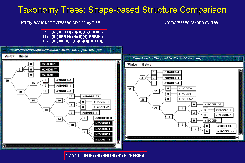
The above figure shows two representations of a taxonomy tree of 50 suboptimal structures of sequence m2, 201 nucleotides long, folded by MFOLD - a Dynamic Programming Algorithm (DPA) - and clustered based upon heuristic measures of similarity among the structures' tree lists. The tree lists are shown in the red boxes above and below the left taxonomy window and correspond to the structures listed in the black nodes in the tree. Please, see the discussion in the Tools Connections section below for further explanations.
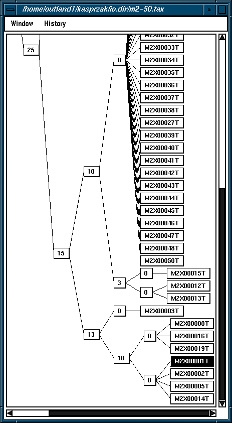
The need for a compressed representation of a taxonomy tree (above right) is stressed by the size of the figure shown below, which is of the same taxonomy tree. It is a totally explicit, or uncompressed, representation where every node is labeled with the name of the particular secondary structure from the solution space examined.


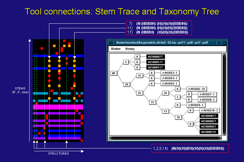
In the above figure the black taxonomy tree nodes and their corresponding tree lists (in the red boxes) are also depicted in a stem trace plot (left) of the first 20 suboptimal structures (from the total of 50 considered in the taxonomy tree). For more information on stem traces click here.
The optimal (1-st) and 2-nd, 5-th, and 14-th suboptimal structures all have the same tree list representation (shown in the bottom red box). As a result, they are clustered in one taxonomy tree node with a heuristic distance measure of 0. On the other hand, they do differ from each other, having unique stems, which is clearly visible in the stem trace of the same data (green, vertical, dashed lines intersect all the component stems of individual structures belonging to this taxonomy tree cluster). The subtree of the 7-th, 11-th, and 17-th suboptimals shows a distance of 3 among them, which is due to different arrangements of Bulge (B) and Internal (I) loops in a the first sublist of their tree list representations (shown in the top red box). In addition to these differences, the structures from this subtree also differ in their component stems (yellow, vertical, dashed lines intersect all the component stems of individual structures belonging to this taxonomy tree cluster).
The relative differences between the two highligthed clusters of structures are clearly visible in the taxonomy tree's distance of 80 between them. They also stand out in the stem trace representation of the solution space. In general, however, the Taxonomy Tree algorithm can be far more sensitive to structureal differences than the Stem Trace depictions.

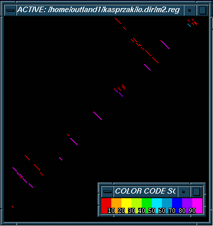
This figure is of a stem histogram that corresponds to the m2 taxonomy trees and the stem trace shown above. It is displaying the top 50 suboptimal structures shown in the the taxonomy trees. In this representation long linear sets of diagonals correspond to non-branching segments in the tree list representations. In contrast to a stem trace representation, the clustering of similar structures is not evident.
For more information on stem histograms click here.